TIPS: Cost of Implicit Nonlinear Analysis
Parallel Computing in Marc
Marc supports parallelisation of
both the element loops and the equation solution.
They are controlled by two
different mechanisms – one of them is “free”, the other requires an additional
license (or FEATURE used from MSC One tokens). Which one is most effective for a
particular analysis will be the subject of another blog entry.The following sections show the two controlling options in the Mentat GUI, and then the results of a benchmark to show the speed obtained using different solvers in combination with parallelisation.
Enabling Parallel Processing
There are two parts to control that are displayed in Mentat:

In the flowchart below, the yellow boundary show the element loops that are affected by DDM, and the green boundary show the matrix solution phase that is controlled by solvers such as Pardiso:
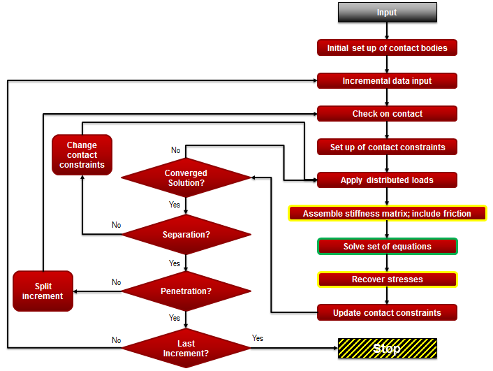
- DDM via –nps run_marc option
- Solver via –nthread run_marc option
Example Comparisons
The following is an example of the speedups achieved with parallel processing. It is a simple model made from 4 touching contact bodies with a basic loading, but deliberately made rather ill-conditioned via some inadequate boundary conditions.

- # Elements 583,200
- # Nodes 629,356
- Element Type 7
- # Contact Bodies 4
- # Increments 5
The results from a few different parallel process analyses are shown in the graphs below:


It is interesting to note that the GPGPU performance is only slightly faster than when using nthread 2 and is 3 times slower than the nthread+nps solution. This is more to do with the Paradiso solver being highly optimised over recent years.
Using the iterative method (CASI), the performance is consistently faster than its nearest and fastest competitor by a factor of 2.3 for ill-conditioned systems and 4.6 for well-conditioned systems.
The memory usage for CASI is also 3.5 times less than its nearest and fastest direct competitor. The use of nps causes a memory requirement increase of 30% over 8 threads, but there is an initial jump in memory requirement of 15% when moving to nps 2 – after this, the increase is low at around 3-4%. Looking at the solving threads, the use of nthread causes a marginal increase in memory requirements (3%)
For domain decomposition, the default metis composer and options within Marc actually work very well with this analysis in general. Changing to vector, fine graph, detect contact etc. made very little difference to the speed for tests that used the direct solvers. The scaling of CASI is more dependent on the domain decomposition than the direct solvers. Typically nps=2 (and 6) gives a sub-optimal performance increase, for example. The scaling for CASI is generally the worst, but it is able to reach the same scaling as an nthread-only analysis as nthread increases.
Overall, the scaling is optimum when using nthread and nps and specifying the number of threads equal to the number of physical sockets.
Scaling beyond the physical number of cores becomes negligible – that is, hyper-threading is of no use to such demanding applications as finite element analysis! Also when using practically all the physical memory has some degradation, but interestingly quite insignificant.
We have also noted that the scaling is better for HEX8 (x5) than for TET4 (x4) elements
In the end, wall time is the key results – and CASI is supreme, even for ill-conditioned problems
More to come!
